Domain colouring: how to see a complex function

The problem

A complex number z = x + iy is a point in the plane. A complex function w = f(z) sends each point of one plane to a point of another. To draw the graph, the set of pairs (z, f(z)), you would need two dimensions for z and two more for w. We can’t draw four dimensions, so we need to give something up.

Domain colouring keeps the input plane as the picture and encodes the output at each point as a colour. Every pixel of the image is a value of z; its colour tells you f(z).

Hue for the angle, brightness for the size

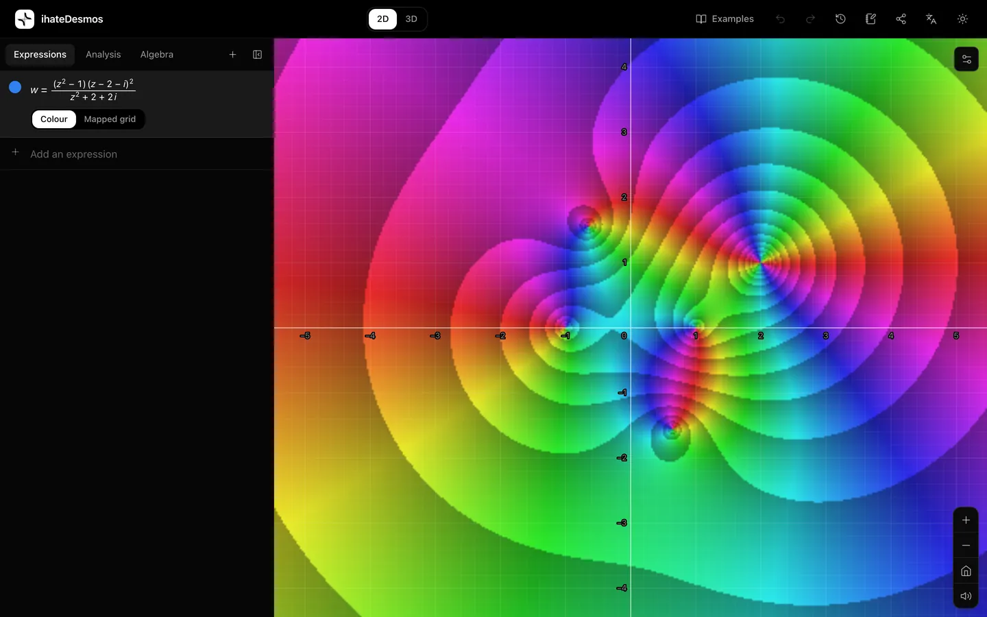
Write the output in polar form, w = |w| e^(iθ). It has a size |w| and an angle θ, called the argument. The standard colouring:

• Hue shows the argument. Red for θ = 0 (positive real numbers), then yellow, green, cyan, blue and magenta as θ goes round, back to red at 2π.
• Brightness bands show the size. Each band is one step in log |w|, so |w| doubles (or grows by some fixed factor) from one band to the next. The bands are contour lines of the modulus.

Reading zeros and poles

Points where every colour meets are where the argument is undefined: zeros (w = 0) and poles (w = ∞). You can tell them apart by the order of the colours as you go round the point anticlockwise:

• Around a zero, the colours run red → yellow → green → blue → magenta, the same direction you are going.
• Around a pole, they run in reverse.
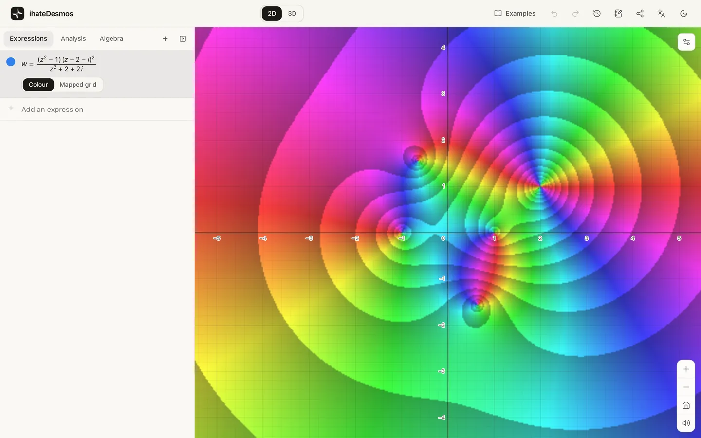
• The number of times the colour wheel repeats tells you the order. Around the double zero at 2 + i in the picture above, the colours go round twice.

The brightness bands help too: they crowd together near zeros and poles, because |w| changes fastest there.

This is the argument principle made visible. Walk around any closed loop in the picture and count how many times the colours cycle: the answer is the number of zeros inside minus the number of poles, each counted with multiplicity.

Mapped grids: watching shapes deform

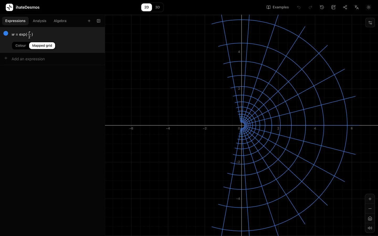
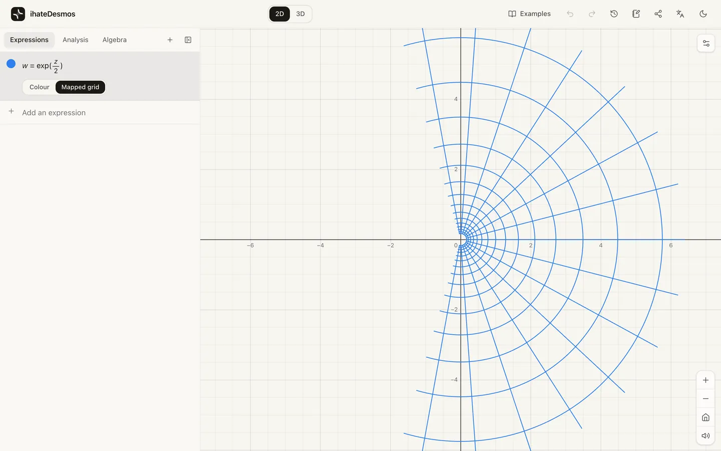
A second way to see a complex function is to draw the image of a square grid. Each horizontal and vertical line of the input plane becomes a curve in the output plane. For an analytic function the image curves still meet at right angles wherever f′(z) ≠ 0. This is what “conformal” means: the map preserves angles locally, even while it bends and stretches everything.

Branch cuts

Some functions, such as √z and ln z, have more than one possible value at each point. A calculator has to choose one, and the choice jumps somewhere: usually along the negative real axis. In domain colouring this shows up as a sudden change of colour along a line, a branch cut. Graph w = sqrt(z) and you will see the colours jump as you cross the negative real axis. The full multi-valued function is better pictured as a Riemann surface, which the 3D mode can draw.

A little history

The idea of colouring the domain goes back decades, and the name “domain coloring” was popularised by Frank Farris in the late 1990s. Elias Wegert’s 2012 book Visual Complex Functions developed it into a systematic way of reading complex analysis from pictures, and it is now one of the standard ways to teach the subject.

Try it

In the calculator, any expression in z with w = on the left is drawn as a complex function. Start with w = z^2 (the colours go round twice), then w = 1/z (a pole: reversed colours), then w = sin(z) (zeros along the real axis). Switch between colour and mapped grid in the row’s options.